.ipynb .pdf

repository

Contents

9. Cloudy vs. clear prediction

9.1. Setup

%load_ext autoreload
%autoreload 2

import glob as glob
import matplotlib as mpl
import matplotlib.patheffects as PathEffects
import matplotlib.pyplot as plt
import matplotlib.transforms as transforms
import numpy as np
import pandas as pd
import seaborn as sns

import corner
import json
import pathlib
import pickle
import utils
import warnings

from astropy import constants as const
from astropy import units as uni
from astropy.io import ascii, fits
from astropy.time import Time
from mpl_toolkits.axes_grid1 import ImageGrid

# Default figure dimensions
FIG_WIDE = (11, 5)
FIG_LARGE = (8, 11)

# Figure style
sns.set(style="ticks", palette="colorblind", color_codes=True, context="talk")
params = utils.plot_params()
plt.rcParams.update(params)

9.2. Dowload data

Unzip this into a folder named data in the same level as this notebook

9.3. Load

df_wakeford = pd.read_table(
    "data/cloudy_vs_clear/H2O_J_data.txt", header=1, sep="\s+", index_col="Name"
)
display(df_wakeford.head())
df_wakeford.dtypes

	T	logg	H2O-J	H2O-J_unc
Name
GJ436	669.0	3.10	0.339500	0.266522
GJ1214	547.0	2.94	0.003296	0.056763
HAT-P-01	1322.0	2.93	1.337013	0.679367
HAT-P-11	838.0	3.06	2.499212	0.504664
HAT-P-12	955.0	2.75	0.217148	0.650651

T            float64
logg         float64
H2O-J        float64
H2O-J_unc    float64
dtype: object

df_wakeford

	T	logg	H2O-J	H2O-J_unc
Name
GJ436	669.0	3.10	0.339500	0.266522
GJ1214	547.0	2.94	0.003296	0.056763
HAT-P-01	1322.0	2.93	1.337013	0.679367
HAT-P-11	838.0	3.06	2.499212	0.504664
HAT-P-12	955.0	2.75	0.217148	0.650651
HAT-P-17	792.0	3.11	1.510989	0.672787
HAT-P-18	841.0	2.73	1.644092	0.401364
HAT-P-26	1001.0	2.65	1.384714	0.239845
HAT-P-32	1801.0	2.78	1.109273	0.395724
HAT-P-38	1082.0	2.99	1.587813	0.550770
HAT-P-41	1941.0	2.84	0.830380	0.198130
HD97658	757.0	3.15	0.387267	0.617148
HD189733	1191.0	3.34	1.914968	0.366223
HD209458	1459.0	2.97	1.201088	0.135370
WASP-6	1184.0	2.90	0.971666	0.386287
WASP-12	2580.0	3.02	1.424847	0.310041
WASP-17	1755.0	2.53	2.312078	0.926330
WASP-19	2077.0	3.16	1.426730	0.532266
WASP-31	1575.0	2.70	0.591729	0.396906
WASP-39	1166.0	2.63	1.241439	0.250035
WASP-43	1440.0	3.70	1.144747	0.522718
WASP-52	1315.0	2.84	1.253270	0.118420
WASP-63	1540.0	2.62	0.779067	0.288147
WASP-67	1003.0	2.93	0.945215	0.767270
WASP-69	963.0	2.73	0.212735	0.092289
WASP-74	1910.0	3.02	0.954418	0.254206
WASP-76	2160.0	2.72	0.732639	0.555734
WASP-79	1716.0	2.92	0.659614	0.598546
WASP-80	825.0	3.16	0.377167	0.262816
WASP-101	1560.0	2.76	-0.341726	0.371857
WASP-107	736.0	2.49	0.602586	0.080241
WASP-121	2358.0	2.97	1.034493	0.264364
WASP-127	1400.0	2.33	1.135027	0.110355
XO-1	1204.0	1.66	0.376148	0.666316

df_southworth = pd.read_table(
    "https://www.astro.keele.ac.uk/jkt/tepcat/allplanets-csv.csv",
    sep=r"\s*,\s*",
    engine="python",
    index_col="System",
)
display(df_southworth.head())
df_southworth.dtypes

	Teff	err	err.1	[Fe/H]	erru	errd	M_A	errup	errdn	R_A	...	errup.8	errdn.6	rho_b	errup.9	errdn.7	Teq	err.2	err.3	Discovery_reference	Recent_reference
System
55_Cnc_e	5172	18	18	0.35	0.10	0.10	0.873	0.051	0.035	0.954	...	2.1	1.9	4.71	0.56	0.53	2349.0	188.0	193.0	2011ApJ...737L..18W	arXiv:1908.06299
pi_Men	5998	62	62	0.09	0.04	0.04	1.070	0.040	0.040	1.170	...	1.9	9.5	2.10	0.40	0.40	1170.0	2.8	4.3	arXiv:1809.05967	arXiv:2007.06410
AD_3116	3184	29	29	0.14	0.10	0.10	0.276	0.020	0.020	0.290	...	-1.0	-1	-1.00	-1.00	-1.00	1669.0	244.0	258.0	2017ApJ...849...11G	2017ApJ...849...11G
AU_Mic_b	3700	100	100	-1.00	-1.00	-1.00	0.500	0.030	0.030	0.750	...	-1.0	-1	-1.00	-1.00	-1.00	-1.0	-1.0	-1.0	arXiv:2006.13248	arXiv:2012.13238
AU_Mic_c	3700	100	100	-1.00	-1.00	-1.00	0.500	0.030	0.030	0.750	...	-1.0	-1	-1.00	-1.00	-1.00	-1.0	-1.0	-1.0	arXiv:2012.13238	arXiv:2012.13238

5 rows × 42 columns

Teff                     int64
err                      int64
err.1                    int64
[Fe/H]                 float64
erru                   float64
errd                   float64
M_A                    float64
errup                  float64
errdn                  float64
R_A                    float64
errup.1                float64
errdn.1                float64
loggA                  float64
errup.2                float64
errdn.2                float64
rho_A                  float64
errup.3                float64
errdn.3                float64
Period                 float64
e                      float64
errup.4                float64
errdown                float64
a(AU)                  float64
errup.5                float64
errdown.1              float64
M_b                    float64
errup.6                float64
errdn.4                float64
R_b                    float64
errup.7                float64
errdn.5                float64
g_b                    float64
errup.8                float64
errdn.6                 object
rho_b                  float64
errup.9                float64
errdn.7                float64
Teq                    float64
err.2                  float64
err.3                  float64
Discovery_reference     object
Recent_reference        object
dtype: object

It seems that something went wrong with the conversion of the errdn.6 column (it should be a float since it corresponds to the lower bound on the uncertainty of g_b), so let’s take a look at what happened:

problem_col = "errdn.6"

# Collect the name (indexed by System name) of each row that fails the conversion check
problem_rows = []
for i, s in df_southworth.iterrows():
    try:
        float(s[problem_col])
    except ValueError:
        print(f"Could not convert {s[problem_col]} to float at ({i}, {problem_col})")
        problem_rows.append(i)

problem_rows

Could not convert 2..9 to float at (K2-060, errdn.6)

['K2-060']

It looks like some badly formatted data snuck in to the column for K2-060. It could be that the value should be 2.9 instead of 2..9, but since we already have so much other data, let’s just play it safe and drop this row:

df_southworth_cleaned = df_southworth.drop(problem_rows)

Now we can continue with the producing the final figure:

logg_wakeford, Teq_wakeford, H2O_J = df_wakeford[["logg", "T", "H2O-J"]].T.values
g_pop, Teq_pop = df_southworth_cleaned[["g_b", "Teq"]].T.values.astype(float)

9.4. Plot

"""
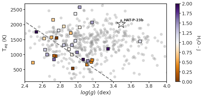
Updated Stevenson+ 16 plot using the H2O-J measurements from 
Wakeford+ 2019
"""
fig, ax = plt.subplots(figsize=FIG_WIDE)

# Plot catalog targets
g_pop_pos_idxs = g_pop > 0.0  # Avoid taking log of invalid nums
logg_southworth = np.log10(100 * g_pop[g_pop_pos_idxs])  # log10(SI -> CGS)
T_eq_southworth = Teq_pop[g_pop_pos_idxs]
ax.plot(
    logg_southworth,
    T_eq_southworth,
    "o",
    color="gray",
    alpha=0.3,
    zorder=-10,
    ms=10,
    mew=0,
)

# Plot H2O-J information
points = ax.scatter(
    logg_wakeford,
    Teq_wakeford,
    c=H2O_J,
    marker="s",
    s=100,
    edgecolor="k",
    cmap="PuOr",
    vmin=0,
    vmax=2,
)
cbar = plt.colorbar(points)
cbar.set_label("H$_{2}$O - J", fontsize=16, labelpad=30, rotation=270)

# Plot HAT-P-23b for context
targ_coords = (3.485, 2027)
ax.scatter(
    *targ_coords,
    c="#F3F3F3",
    marker="*",
    s=1000,
    edgecolor="k",
    cmap="PuOr",
    vmin=0,
    vmax=2,
)
ax.annotate(
    "HAT-P-23b",
    xy=targ_coords,
    xytext=(10, 10),
    textcoords="offset points",
    # ha = "left",
    fontsize=12,
    weight="bold",
)

# Plot WASP-50
# targ_coords = (np.log10(100*30), 1381)
# ax.scatter(
#     *targ_coords,
#     c="g",
#     #marker="*",
#     s=200,
#     lw=0,
#     #cmap="PuOr",
#     vmin=0,
#     vmax=2,
# )
# ax.annotate(
#     "WASP-50b",
#     xy=targ_coords,
#     xytext=(10, 10),
#     textcoords="offset points",
#     ha = "right",
#     fontsize=12,
#     weight="bold",
# )

# Jupiter
# targ_coords = (np.log10(100*25), 150)
# ax.scatter(
#     *targ_coords,
#     c="r",
#     #marker="*",
#     s=200,
#     lw=0,
#     #cmap="PuOr",
#     vmin=0,
#     vmax=2,
# )

# Plot WASP-43
# targ_coords = df_wakeford.loc["WASP-43"][["logg", "T"]].values
# ax.annotate(
#     "WASP-43b",
#     xy=targ_coords,
#     xytext=(10, 10),
#     textcoords="offset points",
#     #ha = "right",
#     fontsize=12,
#     weight="bold",
# )
    
    
# Plot HD189733
# targ_coords = df_wakeford.loc["HD189733"][["logg", "T"]].values
# ax.annotate(
#     "HD189733",
#     xy=targ_coords,
#     #xytext=(10, 10),
#     #textcoords="offset points",
#     #ha = "right",
#     fontsize=12,
#     weight="bold",
# )

# Plot divide
m = (300 - 2100) / (3.3 - 2.4)
loggs = np.linspace(*ax.get_xlim(), 100)
Teqs = m * (loggs - 2.4) + 2100
ax.plot(loggs, Teqs, ls="dashed", lw=3, color="grey")

# Save
ax.set_xlim(2.4, 4.0)
ax.set_ylim(100, 2_700)
ax.set_xlabel("$log(g)$ (dex)")
ax.set_ylabel("T$_{eq}$ (K)")
fig.set_size_inches(FIG_WIDE)
utils.savefig("../paper/figures/cloudy_vs_clear/cloudy_vs_clear.pdf")

8. Retrieval transmission spectra 10. 2D Spectra